Cobe 2.0
Or, it is what it is what it is what it is what it is what it is what it is.
By peter on September 19, 2011 | Permalink
I’m releasing Cobe 2.0, with a major conceptual change in its data model and a more flexible scoring system. To explain the changes, let’s get a little deeper into Cobe 1.x.
Cobe 1.x
When Cobe 1.x learns an input phrase, say “this is a test”, it does the following:
First, it splits the phrase into tokens. Each series of alphanumeric characters becomes its own token, and each series of characters between those becomes another.
So “this is a test” becomes seven tokens:

Cobe 1.x groups these tokens by the Markov Order m (default five) and adds special END tokens that signal the beginning and end of a phrase:
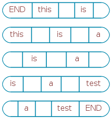
And then each group is annotated with the next token that follows.
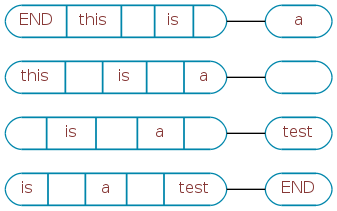
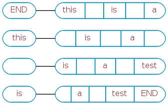
And the previous token:
As more phrases are learned, Cobe keeps track of all the words that have ever followed these contexts. After a while, one might look like:
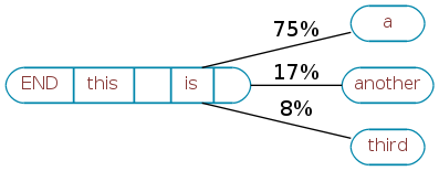
Here you can also see each link annotated with its probability in the learned text. For phrases beginning “this is ”, “this is a” occurred 75% of the time, “this is another” occurred 17% of the time, and “this is third” occurred 8%.
When generating a reply, cobe 1.x picks a random next word, shifts it into the context, and looks for the words that follow that new context.
In functional terms, this works exceedingly well. But there’s no denying that it’s complex. Each context is clearly related to all of the others, but they’re not explicitly connected to each other—the connections are to the next word.
Maintaining the forward and backward chains independently means it’s difficult to visualize the brain as a whole, and since spaces are separate tokens, half of the useful context is taken up tracking whitespace.
Cobe 2.0
Cobe 2.0 employs two major changes to brain storage that reduce complexity, ease visualization, enhance processing speed, and leave us able to use a world of existing general-purpose algorithms.
My first change was to connect contexts directly to each other. Since each is already stored in the database, this is just a matter of creating a table that links the previous context to its next context.
Astute readers will note that this creates a graph. Each context is a graph node, and the graph’s edges are the links between them. Using a directed graph, Cobe ends up learning “this is a test” like this:
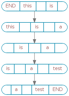
Take note: since the edges of the graph are directed, this same data structure can be used to walk either forward or backward. No more training two chains!
At this point, we’re still looking at the equivalent of a 5th order Markov chain. I wanted to reduce the Markov order by eliminating the whitespace that’s being stored in the contexts.
The other Markov-based chatbots have taken different strategies here. They may group spaces and punctuation together as the tokens that separate words, like Cobe 1.x. They may tokenize punctuation and spaces separately, but still consider spaces as normal tokens. They may attach the spaces as leading or trailing properties of words and reconstruct the spaces when joining the words back together.
Cobe 2.0 takes a different strategy. It eliminates all spaces from the nodes and makes them a property of the graph edges. Combined with the graph layout, this is a major breakthrough. It keeps the database size small and the nodes much more dense with information.
Below is a dump of a 2nd order Cobe 2.0 brain that has been trained with four phrases:
- this is a test
- this is another test
- another test would help
- hal hal hal
The empty node at the top is a special node which signals the end of the graph. It serves the same purpose as the special END tokens in Cobe 1.x. Open arrowheads show nodes that were learned with spaces between them.
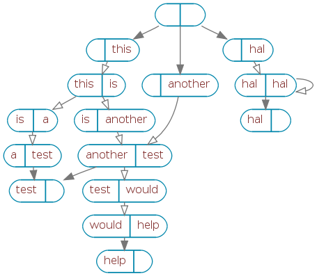
Looking at this, you can easily see how a reply might be generated. Cobe follows a random arrow from every node, building a list of reply words as it goes.
When generating a reply with 2.0, all of the database queries are on the edges table alone. It doesn’t even matter what Markov order the contexts are anymore. Indeed, different contexts could have different numbers of tokens. “Raining cats and dogs” could be identified as a single concept (or collocation), and it could be treated as a single word for replies.
If you follow the graph above, it’s clear that you could get a reply like “this is another test would help” or “hal hal hal hal hal hal hal hal hal hal hal”.
Being able to say quantitatively that the first is a bad reply and the second is a great reply is a question for reply scoring, and I’ve made the groundwork for some changes there too.
Scoring changes
Cobe (both old and new) will generate as many replies as possible during half a second. These are evaluated by a scoring routine, which determines which of the candidates is best. At the end of the half second, the best candidate so far becomes the result.
Cobe 1.x used a scorer based on MegaHAL’s evaluate_reply(), which adds together the self-information of all reply tokens that also appeared in the input. This means that more surprising replies score higher.
MegaHAL’s scorer then applies a couple of dividers to discourage overly long replies.
Recently I’ve been looking more closely at the candidate replies. Many of them are subjectively better than the result, and I’d like to explore scoring for the next few releases.
For Cobe 2.x, I have introduced reply scoring based on several signals. The information content of a reply is one good metric, but there are a lot of other things that might contribute to a good reply. Some examples:
- discouraging overly lengthy replies (as exhibited by MegaHAL’s scorer)
- discouraging replies that are too similar to the input
- discouraging replies that are too similar to the last N responses
- encouraging excited or shouting replies
- encouraging double entendre
- encourage (discourage?) replies that loop back on themselves
- preserve word sense as found in the input
There’s a lot of room for playing around with scoring.
Performance
Cobe 2 is quite a bit faster than 1.x, and a Cobe 2 brain is roughly half the size of the same 1.x brain.
Learning the Brown Corpus, 500 samples of English language text, Cobe 2.0 is about five times faster than 1.2. I adjusted the Cobe 1.2 code to use the same database parameters as 2.0, to get a more accurate comparison of the core learning algorithm:
Cobe 1.2 (adjusted) - 224M brain file
real 18m25.908s
user 5m6.115s
sys  0m36.146s
Cobe 2.0 - 102M brain file
real 3m24.447s
user 2m35.319s
sys  0m19.854s
Reply speed is difficult to measure, as it’s dependent on random factors, but I’m seeing at least double the number of candidate replies in the new code.
My largest brain in production has learned about 230,000 phrases, for 1.8 million edges between 1.4 million nodes. This is better than Cobe 1.x could manage, but there’s still room for improvement. Learning one million phrases is my next scaling goal.
Next steps
Where to go from here?
First, explore new scorers. There are a few listed above, plus general purpose ideas like a Bayesian classifier scorer. That would allow you to train Cobe based on a list of good and bad replies.
The scorers are sometimes at odds with each other—you might want to encourage reply length in one case, brevity in another. It might make sense to build reply profiles out of a set of weighted scorers and score each set of candidate replies based on a randomly chosen profile. (e.g. “SHORT AND SHOUTY” or “long and repeating and repeating and repeating and repeating and repeating”)
Second, continue improving the speed of candidate replies. Assuming the scorers are going to select the best response, Cobe needs to make candidates as quickly as possible.
I have two strategies planned for faster replies. Currently, Cobe performs a random walk from scratch for every candidate. This could be made a lot faster by turning the walk into a generator, searching the tree for the END token and yielding a reply every time it’s found.
The second strategy is to start generating replies in parallel. Cobe is easily distributed across a large number of computers.
Have fun out there.


